Markov Decision Process & QLearning

Reinforcement learning is a framework for teaching agents to make decisions in complex environments. At the core of this approach is the idea of a Markov Decision Process (MDP), which is a way of describing situations where an agent makes decisions in an environment that’s a mix of chance and control. One of the most well-known algorithms for solving MDPs is Q-Learning, a model-free method that enables agents to learn optimal actions through trial and error, without requiring a full model of the environment.
This post covers a two-part project. In the first part, I implemented a simulation where an agent navigates a grid-world environment, aiming to reach a goal state while avoiding obstacles. In the grid-world, the agent can move up, down, left, and right. Each move incurs a cost, and the objective of the agent is to minimize the total cost while reaching the goal.
The agent will move using an algorithm that utilizes the Bellman equation, value iteration algorithm, and Markov decision process (MDP) framework. These concepts enable simulating the agent’s traversal. A reward system assigns a cost of -1 per move and a reward of +100 for reaching the goal. The total expected return (sum of costs and rewards) is optimized using value iteration.
The Bellman equation is used to compute the optimal value function for each state in the MDP:
\[V(s) = \max_a \left( R(s, a) + \gamma \sum_{s'} T(s, a, s') \cdot V(s') \right)\]Where:
- \(V(s)\) is the value function for state s, which represents the expected total cost of reaching the goal state from that state.
- \(\max_a\) is the maximum over all possible actions a in state s (the optimal policy).
- \(R(s, a)\) is the immediate reward received for taking action a in state s.
- \(\gamma\) is the discount factor, which determines the importance of future rewards relative to immediate rewards. This can be set to a relatively high value ~0.9 in order to encourage the agent to reach the goal state as efficiently and quickly as possible.
- \(\sum_{s'} T(s, a, s') \cdot V(s')\) is the expected discounted value of the future rewards (next state)
By computing the optimal value function using the Bellman equation, we can determine the optimal policy (i.e., the optimal sequence of moves) for the agent to reach the goal state with the lowest possible total cost. The agent can follow this policy to navigate the grid-world environment and reach the goal state while avoiding obstacles.
The grid-world environment is created using a custom grid system with sprites. Each cell represents a state in the Markov decision process (MDP) and is labeled with an ID or coordinate. The object’s action options (moving up, down, left, or right) on the grid correspond to the actions in the MDP and can be represented by integers.
Transition probabilities from one state to another depend on the grid’s structure and obstacles. They are defined using a transition function that takes the current state and action as input, returning the next state and its probability. The reward function determines the immediate reward for each action, and will be defined using a function that takes the current state and action as input and returns the corresponding reward.
To implement value iteration, the MDP script includes a function that computes the optimal value function and policy for each state. The value function will be initialized to 0 and will be updated at each iteration using the Bellman equation. Once the value iteration algorithm converges, the optimal value function can be used to determine the optimal policy for each state in the MDP. Then, we can control an object’s movement using the policy.
FlowChart:
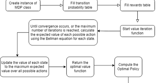
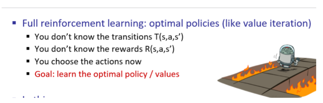
The goal of the second part of this project was to adapt the previous program, which solves an MDP using value iteration, to instead incorporate machine learning techniques. To do so, I followed these steps:
- Choose a learning algorithm: This involves selecting a learning algorithm that can learn from the MDP. This may involve selecting a reinforcement learning algorithm, such as Q-learning or SARSA.
- Train the model: Train the model by repeatedly simulating the MDP and updating the policy based on the observed rewards. This involves running the learning algorithm on the MDP until the policy converges.
- Tune the parameters: The parameters of the model, such as the learning rate or discount factor, can be modified to make the agent behave as desired. For example, using a small discount factor will cause the agent’s optimal policy to converge towards immediate rewards.
Machine learning algorithms like Q-learning enable an agent to learn and adapt to an environment without requiring prior knowledge. This capability makes Q-learning widley applicable to real-world scenarioes like games, robotics, and autonomous vehicle navigation.
Q-learning is a model-free reinforcement learning algorithm that trains an agent in an MDP environment. It is a type of adaptive dynamic programming, which is a category of machine learning algorithms that are used to solve optimization problems in dynamic environments. The agent starts with no prior knowledge of the MDP’s transition or reward functions, and learns an optimal policy that maximizes the expected cumulative reward over time through exploring the environment.
At each time step, the agent observes the current state of the environment, chooses an action, and receives feedback from the environment in the form of a reward and a new state. Over time, the agent updates its understanding of state-action pairs using the Q-values, which represent the expected cumulative reward of taking a specific action in a given state while following the optimal policy thereafter. The updates rely on the Bellman equation, which calculates the Q-value as the immediate reward plus the discounted maximum Q-value of the following state-action pair. The Q-values are refined iteratively through exploration and converge to optimal values. The agent then selects actions based on the Q-values of the current state, following a policy that is greedy with respect to the learned Q-values.
The MDP implementation in the fist part of this project uses a predefined transition and rewards function. To modify the program to use Q-learning, I need to implement a Q-learning algorithm, which will update the Q-values based on the observed rewards and choose actions based on the highest Q-values. Using this approach, the agent should learn an optimal policy without complete knowledge of the entire environment.
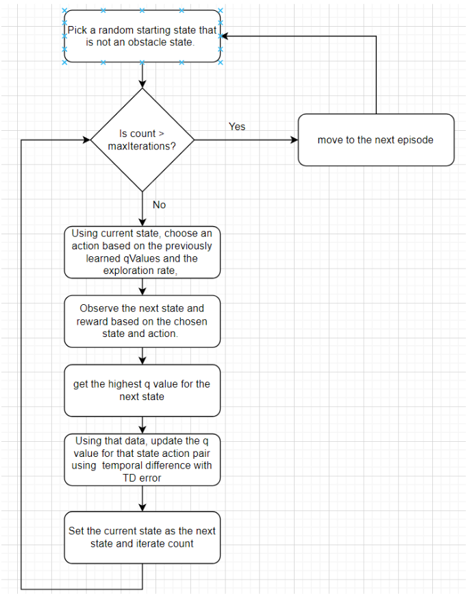
Here is the main loop for interatively refining the Q-values. We let the agent have a lifetime of a given number of moves to simulate an episode. With each episode, the agent uses the updated Q-values for state-action pairs from the previous trial to explore the environment.
public void QLearning(int numEpisodes, int maxIterations, int getPolicyOnEpisode)
{
    for (int episode = 0; episode < numEpisodes; episode++)
    {
        int state = UnityEngine.Random.Range(0, numStates);

        while(IsObstacleState(state))
        {
            state = UnityEngine.Random.Range(0, numStates);
        }

        if (episode % getPolicyOnEpisode == 0)
        {
            startingStateList.Add(state);
        }

        int count = 0;
        while (count < maxIterations)
        {
            int action = ChooseAction(state);

            (int nextState, float reward) = GetNextStateAndReward(state, action);

            float maxQValue = GetMaxQValue(nextState);

            //update qValue using temporal difference error

            //qValues[state,action] is the current estimate of Q-values
            //alpha is learning rate
            //reward is the reward obtained by taking action in that state
            //gamma is the discount factor (imporatance of future rewards vs immediate rewards)
            //maxQValue is the maximum QValue amoung all possible actions in the next state.
            qValues[state, action] = qValues[state, action] + alpha * (reward + gamma * maxQValue - qValues[state, action]);

            state = nextState;

            if(reward == obstacleReward)
            {
                break;
            }

            count++;
        }

        // Every xth episode, add the current policy to the list
        if (episode % getPolicyOnEpisode == 0)
        {
            int[] policy = GetOptimalPolicy();
            policyList.Add(policy);
        }

    }
}
At each step, the agent selects an action using an ε-greedy strategy. Either the agent explores with probability ε, or exploits by selecting the action with the highest Q-value. The ε property helps the agent balance between exploration and exploitation, which ensures that the agent discovers better strategies while still using what it has already learned.
private int ChooseAction(int state)
{
    // Choose a random action with probability epsilon
    // else choose the action with the highest Q-value for the current state with probability 1-epsilon

    if (UnityEngine.Random.Range(0.0f, 1.0f) < epsilon)
    {
        // Choose a random action (exploration)
        return UnityEngine.Random.Range(0, numActions);
    }
    else
    {
        // Choose the action with the highest Q-value for the current state (exploitation)
        float[] qValuesForState = new float[numActions];
        for (int i = 0; i < numActions; i++)
        {
            qValuesForState[i] = qValues[state, i];
        }
        return Array.IndexOf(qValuesForState, qValuesForState.Max());
    }
}
Once an action is chosen, the reward for that state and chosen action is acquired through a lookup in the predefined reward table, and a check ensures the next state is valid.
private (int, float) GetNextStateAndReward(int state, int action)
{
    int nextState = GetNextState(state, action);

    if (nextState == -1)
    {
        Debug.Log("nextState = -1");
        return (state, obstacleReward);
    }
    else
    {
        // Retrieve the reward from the predefined reward table
        float reward = rewards[state, action, nextState];
        return (GetNextState(state, action), reward);
    }
}
To update Q-values, the agent needs to estimate the best possible future reward from a given state. This function retrieves the maximum Q-value, via another lookup, among all available actions for the specified state.
private float GetMaxQValue(int state)
{
    // Finds the maximum Q-value among all possible actions in a given state.
    // This helps estimate the best future reward possible from the state.

    float maxQValue = float.MinValue;
    for (int i = 0; i < numActions; i++)
    {
        if (qValues[state, i] > maxQValue)
        {
            maxQValue = qValues[state, i];
        }
    }
    return maxQValue;
}
Once training is complete, we can get the optimal policy by selecting the action with the highest Q-value for each state. This function returns an array where each index represents a state and its corresponding value is the best action to take.
public int[] GetOptimalPolicy()
{
    int[] policy = new int[GetNumStates()];

    // For each state, choose the action with the highest Q-value
    for (int state = 0; state < GetNumStates(); state++)
    {
        float maxQValue = float.MinValue;
        int maxAction = -1;

        // Iterate through all actions and select the one with the highest Q-value
        for (int action = 0; action < GetNumActions(); action++)
        {
            if (qValues[state, action] > maxQValue)
            {
                maxQValue = qValues[state, action];
                maxAction = action;
            }
        }

        policy[state] = maxAction;
    }

    return policy;
}
Then when deciding how to move the agent, the direction from the optimal policy is sampled using the agent’s current position. You can see how after training the agent always uses the optimal strategy, which is to move back and forth to the state with the highest reward.
I think it would be interesting to try and implement reinforcement learning to control enemy AI in a game. I don’t think it would be practical, because it would be difficult to try and ensure that the AI behaves in a predictable or balanced way to ensure a good player experience, though it might still be a valuable learning experience.
To do this, a 2D world would probably be an ideal starting point, since it would simplify the action space and state representation. Given the need for more structured and predictable behavior, I imagine that it would be ideal to use a finite state machine to represent the agent’s different possible actions and states. This would allow for more controlled decision-making, while still enabling some degree of adaptability in enemy behavior that could be trained. For example, using a finite state machine to represent different enemy attacks, and training the agent to know when to use a specific attack in a specific scenario.